Ableton Operator provides a unique hybrid approach to additive, subtractive, and FM synthesis (somewhat like the Synclavier did) and is one of the most deceptively powerful softsynths available.
Even so, many musicians shy away from using it fully because FM synthesis remains opaque despite its prevalence for more than 30 years. Fortunately, Operator’s clean interface and streamlined tools make it the perfect synth for getting started with both FM and additive synthesis, so you can start whipping up your own creations with it.
Operators are standing by
The term operator was first popularized with Yamaha’s groundbreaking DX series of synthesizers, where it was generally defined as being an oscillator with its own dedicated amplitude envelope. In modern FM synthesis, configurations of multiple operators are called algorithms. In a nutshell, algorithms govern the interaction between a set of operators, with each algorithm functioning as its own synthesis structure. If you’re a modular-synth fan, think of them as preconfigured cable routings. That is, each type offers different features that make it well-suited to specific applications.

Because Operator’s features include multiple synthesis options, the easiest way to get started is with the all-carrier algorithm (see Figure 1). While there is no FM functionality here, it’s fantastic for both analogue-style subtractive synthesis and more exotic additive approaches, which should also appeal to fans of vector synthesis. In this algorithm, Operator functions as a four-oscillator synth with individual volume envelopes for each oscillator, followed by a modelled analogue filter. (Note that the filter is at the end of the chain, after each oscillator’s amp envelope. We’ll address this later.)
Tuning details

For newcomers, the nuances of FM tuning are crucial to understanding Operator’s oscillators. Unlike traditional analogue programming, the “coarse” knob tunes the oscillators to specific harmonics and not semitones or octaves, making it essential to understand the note relationships for each harmonic (see Figure 2). For example, the first harmonic is the fundamental, the second is an octave higher, the third is an octave plus a fifth, while the fourth is two octaves above the fundamental. There are numerous online resources for researching the exact relationships, but for getting started in a subtractive context, memorize the octave harmonics: 0.5, 1, 2, 4, 8, 16, 32 and 64.
In another twist, Operator’s fine-tuning knob always spans an octave, divided into 1,000 steps, with positive amounts only. So if you want to apply classic analogue detuning on two oscillators you’ll need to set one oscillator an octave lower, then raise its fine-tuning to between 980 and 999, which results in it being tuned slightly flat by a few cents. For the other oscillator, it’s much easier; simply raise its fine-tuning by a relative amount between 1 and 20. It sounds tricky, but it’s easy to get used to.
For example, to create a four-oscillator detuned supersaw-style patch using the carrier algorithm set two oscillators to a coarse tuning of 1 and the other two to a coarse tuning of 0.5 (sub-octave), then raise the fine-tuning to +995 and +985 on the sub-octaves and +5 and +15 on the fundamentals (see Figure 3).

Additive waveforms
In addition to traditional subtractive waveforms, Operator’s oscillators also include an additive editor with up to 64 partials for each waveform. Any of the preset waveforms can be used as starting points for further editing, but here are two techniques to get you started on your own original waveforms from scratch.

Formant Sculpting. Additive synthesis is useful for digital voice textures, and you can create vowel formants by attenuating or emphasizing specific clusters of harmonics (see Figure 4). Lower clusters correlate with “aahs” and “oohs,” while higher clusters are ideal for “eeee” sounds.

Bell Harmonics. For bell and chime tones, start with the sine waveform as the fundamental and add several widely spaced harmonics (see Fig. 5). These can even be randomly selected, as long as there are only a few and they cover a wide range of frequencies.
ProTip: You can also emphasize a few of these chime harmonics in other waves and create unique hybrid sounds.
Introducing FM

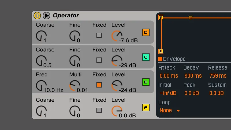
Once you understand the basics of manipulating carriers, it’s time to start adding FM elements. The two algorithms in Figure 6 are perfect starting points for your experiments, with the first offering a single FM modulator simultaneously affecting three carriers. The second algorithm contains two independent carrier oscillators while adding an FM carrier-modulator pair as a secondary element.
Here’s a simple technique that will get you started with the “triple” FM algorithm above. Set all oscillators to sine waves and tune the three carriers to 1, 2, and 4. This will give you an organ-like sound consisting of three octaves. Next, slowly raise the level of oscillator D to around -15dB. As you raise this level, you’ll hear a dramatic harmonic shift in the sound as the frequency modulation for all three carriers becomes more pronounced. This approach is the essence of FM synthesis.
Since every FM oscillator includes its own envelope, you can now manipulate the intensity of the frequency modulation over time—and thus, change the timbre—by adjusting the shape of the modulator envelope. Short envelopes with quick decays are great for percussive tones, while long attacks and releases will deliver results that slowly evolve over time.
After you’ve experimented with the triple-carrier FM algorithm, switch to the algorithm with two carriers and a single FM carrier-modulator pair. Turn off oscillators A/B so you can focus on the C/D carrier-modulator pair, then set its carrier to a sine wave with a coarse tuning of 1 to keep the results consistent.
Two-layer FM

Figure 7 shows my all-time favourite FM algorithm for getting quick results from a 4-operator synth. It consists of dual, independent carrier-modulator pairs and works really well for quickly creating layered effects. For example, you can use the A/B pair for a plucked transient and setup C/D for more of a pad tone. The simplified concept is that the carrier oscillator handles tuning and volume, while the modulator governs the overall timbre and its envelope.
Translating FM terms
Here is a quick way to correlate the parameters of FM and subtractive synthesis when using a single FM oscillator pair.
Carrier Coarse Tuning: Overall pitch
Carrier Level: Volume
Carrier Envelope: Amp Envelope
Modulator Coarse Tuning: Waveshape (e.g. the resulting timbre after FM is applied)
Modulator Level: Filter Cutoff
Modulator Envelope: Filter Envelope
Multiple modulators


Now that we’ve covered the basics of modulators and carriers, let’s take a look at a slightly more sophisticated algorithm that consists of three modulators affecting a single carrier in parallel. In Figure 8, each modulator can affect a different element in your sound. For example, the first modulator can generate the timbre for a sustained tone, the second modulator can introduce a subtle decay sweep, while the third modulator applies a sharp attack transient (see Figure 9).
At this point, it’s important to understand that the tuning and envelope for each modulator dramatically define its role in the end result. By using a low coarse tuning value and level between 1 and 5 for the sustaining modulator, you can create more subdued tones, as higher harmonics with extreme modulation levels impart harshness. The same general approach should be used for the decay-sweep modulator (with a different envelope) as all three modulators interact to create the end result. For the transient modulator with its quick envelope, try tuning it to a very high harmonic for a bright mallet strike effect.
Looping envelopes
This patch is also an excellent starting point for understanding looping envelopes, thanks to its structure. Once you’ve set up the patch described above, turn on envelope looping for the decay-sweep modulator and transient modulator, then tinker with the looping rates for each.
Looping is fantastic for creating complex, rhythmic textures that would be difficult to duplicate in most other softsynths. Fortunately, the principle is straightforward: When looping is turned on, the envelope repeats the attack-decay section as long as the note is held. Adjusting those segments allows for custom LFO-like results or repeating percussive patterns. Depending on which envelopes are looped, you can affect either volume (carrier) or timbral (modulator) elements.
There are five loop modes: None, Loop, Beat, Sync, and Trigger. None turns looping off and the envelope functions normally. Loop sets the repeat rate in millisecond increments up to 20-second intervals. Beat and Sync tie the repeat rate to specific note values that interact with the Live set’s global tempo. Last, Trigger mode is unlooped and causes the envelope to behave as a one-shot that continues through all envelope segments, ignoring note-off events.
Stacked algorithms
Now that you’ve got a solid foundation for understanding how modulators interact with carriers, it’s time for the final set of algorithms. These structures include modulators that interact with other modulators, generating extremely sophisticated timbral results.

As you begin experimenting with stacked algorithms, it’s best to keep all of your oscillators set to sine waves, as they are the easiest to control and yield the most predictable results (see Figure 10). They’re also the basis for Yamaha’s DX line of synths, so as you tinker with Operator, you may stumble across a few classic tones.
Here are three rules of thumb for understanding the functionality for stacked algorithms.
1. If a modulator’s envelope reaches zero, any modulators above it will also be silent, even if they have sustaining envelopes as there is nothing to modulate.
2. Because of this, modulators with sustaining envelopes or long decays should be closest to the carrier, while those with shorter decays should be higher in the algorithm. Simply put, the shorter the decay, the higher it should be in the algorithm.
3. Any modulator at the top of an algorithm also includes its own feedback loop, which can be used for additional spectral complexity.
Oscillator tips
In addition to their waveforms and additive tools, all oscillators include a few additional parameters that can dramatically affect their sound.
Wave: Selects from an array of standard preset waves. The mode switches to “User” if any harmonics are edited.
Repeat: This unusual parameter radically shifts the timbre by repeating the harmonics above the visible display. For example, if you select the 16 or 32 harmonic editors, toggling on Repeat at ¼ or ½ value will add a bit of high-frequency shimmer. The higher values attenuate the repeated harmonics. This feature is great for adding old-school digital shimmer to additive waveforms.
Feedback: If a modulator is at the top of an algorithm, the Feedback parameter will be available. This creates a modulation feedback loop for that oscillator. High levels of feedback add a harsh texture to the sound. With feedback set to maximum, modulators will generate noise if their envelopes are set to full sustain.
Phase: This adjusts the phase for each oscillator’s waveform, with a Retrigger button next to it that restarts the phase with each new trigger. With retrigger off, the oscillators are free-running, useful for approximating analogue behaviour in the all-carrier algorithm.
Osc < Vel: This unusual parameter increases the oscillator tuning frequency in conjunction with velocity. Turning on the Q (quantization) parameter forces the oscillator pitch to one of the coarse harmonics—fantastic for velocity-controlled timbral effects.
Filters

Introduced in Live 9.5, Operator’s filters now include impressive models of three iconic analogue synths and one hybrid variation (see Fig. 11). The model names are abbreviated in the selector pulldown as follows: Oxford OSCar (OSR), Korg MS20 (MS2), Moog Prodigy (PRD) and a hybrid of the OSCar and MS20 (SMP).
While these sound impressive and are useful for beefing up patches (especially in conjunction with the filter drive parameter), there’s an additional detail worth noting: The filter comes at the end of the chain, with no amp section following it.
In most cases, this generally doesn’t pose a problem thanks to the oscillator envelopes. However, because the analogue models are so accurate, high levels of resonance may cause the filter to self-oscillate endlessly. Knowing this will help avoid unexpected sonic mayhem, as self-oscillation can sometimes run amok without an amp envelope to shut down the signal path.
